
DWH: Introduction to BigQuery
DE-zoomcamp course: Module 3

Based on lectures from DataTalksClub and Google BigQuery's official documentation, this introductory overview delves into the architecture and resource organization of Google BigQuery. Exploring the resource hierarchy, dataset patterns, query internals, and best practices, this guide provides insights into effectively organizing and utilizing BigQuery resources for optimal performance and efficiency.
Source:
Google BigQuery’s official documentation
Contents:
Architecture
BigQuery’s architecture is divided into a storage layer for data ingestion and optimization (colossus), and a compute layer for analytics (dremel), operating independently via Google's high-capacity network.
Colossus is Google's advanced distributed file system and the successor to the Google File System (GFS), provides the scalable and reliable storage backbone for Google Cloud services, including BigQuery. It enhances GFS's capabilities with improved data durability and availability through petabyte-scale management and automatic replication.
Dremel is the innovative query service technology that powers BigQuery, enabling fast, interactive analysis of large datasets. It utilizes columnar storage for efficiency and a tree architecture for rapid SQL-like query execution over vast data volumes, leveraging the robust storage capabilities of Colossus.

Capacitor is Google BigQuery's internal storage format, engineered for high-speed analytics. It optimizes query performance through columnar storage, enabling efficient data scans and compression. This format allows BigQuery to read only the necessary data for queries, enhancing speed and reducing resource usage. Capacitor's design, including data clustering by column values, plays a crucial role in BigQuery's ability to offer fast, scalable, and cost-effective data analysis.
BigQuery resources organization
Resource hierarchy
The Google Cloud resource hierarchy, utilized by BigQuery, introduces datasets as an additional layer specific to BigQuery for organizing and controlling access to resources.
Datasets act as logical containers for BigQuery assets like tables, views, functions, and procedures, with the exception of connections and jobs which are linked to projects. Each dataset is defined by a location that cannot be changed post-creation, influencing where table data is stored.
Projects, essential for using Google Cloud services, can house multiple datasets of varying locations.
Jobs, which are operations performed on BigQuery data, are tied to projects but can access tables across multiple projects, with costs billed to the project’s attached Cloud Billing account.
Folders offer another layer of organization above projects, allowing for hierarchical access policy inheritance, while Organizations serve as the top-level entity providing centralized control over resources.
The recommended setup involves creating an Organization resource for overarching management of BigQuery and other Google Cloud resources.

Patterns
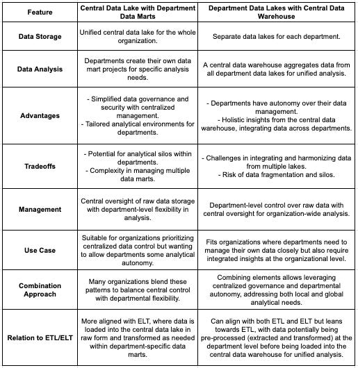
The two patterns for organizing BigQuery resources - central data lake with department data marts, and department data lakes with a central data warehouse - offer different approaches to data management and analysis:
Central Data Lake, Department Data Marts
Central Data Lake: A unified storage for all raw data across the organization.
Department Data Marts: Tailored projects by departments for specific analysis needs.
Advantages: Simplified data governance and tailored departmental analysis.
Tradeoffs: Potential for data silos and complex management of multiple data marts.

Department Data Lakes, Central Data Warehouse
Department Data Lakes: Individual storage projects managed by departments.
Central Data Warehouse: Aggregates data from all departments for unified analysis.
Advantages: Departmental autonomy and organization-wide insights.
Tradeoffs: Challenging data integration and risk of data fragmentation.

Hybrid Approach
Many organizations blend these patterns to balance departmental autonomy with the need for centralized data governance and analysis. This involves maintaining both a central data repository for overarching governance and department-specific projects for localized needs, combined with a central warehouse for comprehensive analysis. The choice between or combination of these patterns depends on the organization's structure, data strategy, and the balance between central oversight and departmental flexibility.organization.
Datasets
Datasets in BigQuery, essential for organizing and controlling access to tables and views, must be created within a specific project before loading data. They are identified using projectname.datasetname in GoogleSQL or projectname:datasetname with the bq command-line tool.
Location: When creating a BigQuery dataset, you set its storage location, which cannot be changed later. However, datasets can be copied or moved to new locations. Queries are processed in the same location as the dataset.
Limitations: BigQuery dataset limitations include
immutable location post-creation
query-referenced tables must share location
copied tables require source and destination datasets in the same location
dataset names must be project-unique
Data retention: Datasets in BigQuery retain deleted or modified data for a short period using time travel and fail-safe features for potential recovery.
Adjust Dataset Settings through various interfaces (console, SQL, bq, terraform etc):
Cross region replication
When creating a BigQuery dataset, you choose a storage location, either a region (a specific geographical area with data centers) or a multi-region (a larger area encompassing multiple regions).
BigQuery stores data in two zones within the chosen location, ensuring zone-level replication but not cross-region redundancy.
Multi-region selection doesn't increase availability during regional outages, as data remains within a single region.
For extra redundancy, datasets can be replicated to a secondary region, creating four zonal copies across two regions through asynchronous replication.

Data retention
Time travel in BigQuery allows accessing data as it was within the last seven days, enabling queries on updated or deleted data, and restoration of tables. The default time travel window is seven days, adjustable from two to seven days at the dataset level, affecting all tables within. Adjusting this window can balance recovery needs and storage costs, with shorter windows reducing costs under the physical storage billing model.
Limitations: Time travel is limited to the set window for accessing historical data. For longer preservation, use table snapshots. Only table administrators can use time travel for tables with row-level access policies. It doesn't restore table metadata.
Fail-safe period retains deleted data for an extra seven days beyond the time travel window for emergency recovery, allowing table-level data recovery at the deletion timestamp. The fail-safe period is fixed and data within it can't be queried or directly accessed; recovery requires contacting Cloud Customer Care.
Dataset contents
Within a BigQuery project, each dataset serves as a collection point for tables and views, potentially encompassing additional datasets to create a structured hierarchy for data organization. The primary elements of a dataset in BigQuery include:
Tables: Fundamental units for data storage, BigQuery tables are analogous to those in traditional relational databases, structured with rows and columns. Each table adheres to a defined schema that specifies its column names and data types, outlining the data's arrangement.
You can find more information on tables here.
Views: Represented as virtual tables constructed from SQL queries, views function as persistently stored queries that you can interact with as though they were standard tables. Rather than storing data, views dynamically produce data from base tables upon access, reflecting the current state of that data.
You can find more information on views here.
Materialized Views: Diverging from conventional views, materialized views hold the query's result set for quicker retrieval, periodically refreshing to mirror updates in the data they derive from.
You can find more information on views here.
Routines: This category encompasses both stored procedures and user-defined functions (UDFs), enabling the execution of sophisticated SQL tasks, logic encapsulation for repeated use, and the facilitation of data calculations and transformations within a dataset.
You can find more information on routines here.
Tables vs Views vs Materialized Views

Query internals
BigQuery query internals encompass the underlying processes that enable efficient query execution within the platform. Powered by a distributed processing engine and columnar storage format, BigQuery efficiently processes queries in parallel across multiple servers. It employs advanced optimization techniques like query parallelization and data pruning to enhance performance. Understanding these internals is key to optimizing query performance and leveraging BigQuery effectively for data analysis tasks.
This subject is thoroughly covered in another dedicated post.
Best Practice
Reducing Costs:
Refrain from using SELECT * in queries.
Estimate query costs before execution.
Implement clustering or partitioning for tables.
Exercise caution with streaming inserts.
Incrementally materialize query outcomes.
Improving Query Performance:
Apply filters to partitioned column data.
Opt for data denormalization.
Utilize nested or repeated columns.
Employ external data sources judiciously; avoid them for high-performance needs.
Minimize data volume prior to executing JOIN operations.
Understand that WITH clauses are not substitutes for prepared statements.
Refrain from creating excessively many shards of tables.
Steer clear of JavaScript user-defined functions.
Implement approximate aggregation functions, such as HyperLogLog++.
Prioritize ordering as the final step in query operations for optimal performance.
Refine your join strategies. Begin with the table that has the highest row count, proceed with the table with the lowest, and arrange any additional tables in descending order of size as a best practice.