
Batch processing: PySpark
DE ZoomCamp course: Module 5

In this brief overview, we delve into batch processing using PySpark, covering essential aspects from data processing types and the Spark engine to practical steps for setting up locally and in the cloud. We touch on initializing SparkSession, DataFrame operations, data selection and transformation, and optimizing processes through partitioning. Additionally, we explore PySpark's integration with SQL for efficient data handling, and the seamless interaction between Spark, Google Cloud Storage (GCS), and BigQuery. This includes creating persistent Spark clusters with Dataproc for scalable cloud-based data processing, aiming to provide a comprehensive guide for leveraging PySpark's capabilities in batch processing tasks.
Sources:
Content:
Data processing types
Batch Processing (80%)
Definition: Processes data in large, single batches at scheduled intervals. Ideal for large volumes of data not requiring immediate feedback.
Technologies: Python scripts, SQL, Apache Spark, Apache Flink.
Advantages: Easy to manage, scalable, retry-friendly.
Disadvantage: Can introduce delays in data processing results.
Workflow: Data Lake → Python script → SQL (dbt) → Spark → Back to Data Lake.
Stream Processing (20%)
Definition: Processes data in real-time as it arrives, suitable for applications needing immediate insights.
Technologies: Apache Kafka (for streaming), Apache Flink, Apache Spark (structured streaming).
Use Cases: Real-time analytics, monitoring systems, instant decision-making applications.
Apache PySpark
PySpark is Apache Spark's Python API, enabling scalable data processing and analysis with Python's simplicity. It supports Spark SQL, DataFrames, streaming, and machine learning, making big data analysis accessible for Python users.

Spark SQL & DataFrames: Mix SQL queries with Spark programs for structured data processing. Supports both Python and SQL with the same execution engine.
Pandas API on Spark: Scale pandas workflows across multiple nodes without changing your code, offering a seamless transition from pandas to Spark for big data.
Structured Streaming: Offers scalable, fault-tolerant stream processing on the Spark SQL engine, allowing for continuous data processing.
MLlib: A scalable machine learning library built on Spark, providing high-level APIs for machine learning pipelines.
Spark Core & RDDs: The foundation of Spark, offering in-memory computing and Resilient Distributed Datasets (RDDs), though DataFrames are recommended for ease of use and optimization.
Spark Streaming (Legacy): A high-throughput, fault-tolerant stream processing extension of Spark Core, now superseded by Structured Streaming.
Spark engine
Definition: An open-source analytics engine for large-scale data processing, supporting batch and stream processing.
Cluster Use: Functions across clusters for distributed computing.
Languages: Supports Java, Scala, Python, R.
Usage Guidance: Opt for SQL (Hive, Presto/Athena) for simple tasks. Use Spark for complex data transformations

Workflow: Raw data → Data Lake → Preprocess with SQL → Process with Spark for complexity → Python for ML training → Store in Data Lake.


Local setup (Linux)
Java Installation for Spark
Requirement: Java 11, compatible with Spark (link with archived versions).
Organization: Create separate folders for Java and Spark.
Download Java 11:
wget https://download.java.net/java/GA/jdk11/9/GPL/openjdk-11.0.2_linux-x64_bin.tar.gz
Extract Java Archive:
tar xzfv openjdk-11.0.2_linux-x64_bin.tar.gz
Set Environment Variables:
Define
JAVA_HOMEand add Java toPATH:export JAVA_HOME="${HOME}/spark/jdk-11.0.2" export PATH="${JAVA_HOME}/bin:${PATH}"
Verify Installation: Run
java --version.Cleanup: Delete the downloaded archive
rm openjdk-11.0.2_linux-x64_bin.tar.gz.Persist Settings: Add
JAVA_HOMEandPATHupdates to~/.bashrcto apply on each session start.
Spark Installation
Version: Use Spark 3.3.2. (link with archived versions)
Download Spark 3.3.2:
wget https://archive.apache.org/dist/spark/spark-3.3.2/spark-3.3.2-bin-hadoop3.tgz
Extract Spark Archive:
tar xzfv spark-3.3.2-bin-hadoop3.tgzSet Environment Variables:
Define
SPARK_HOMEand updatePATH:export SPARK_HOME="${HOME}/spark/spark-3.3.2-bin-hadoop3" export PATH="${SPARK_HOME}/bin:${PATH}"
Verify Installation: Start
spark-shelland run a test script.Cleanup: Remove the archive
rm spark-3.3.2-bin-hadoop3.tgz.Persist Settings: To set
SPARK_HOMEandPATHon bash start, add them to~/.bashrc.
PySpark Installation and Setup
Check Py4J Version: Look for the version of the Py4J file in ${SPARK_HOME}/python/lib/.
Configure PYTHONPATH
Add PySpark and Py4J to PYTHONPATH:
export PYTHONPATH="${SPARK_HOME}/python/:$PYTHONPATH"
export PYTHONPATH="${SPARK_HOME}/python/lib/py4j-[your-version]-src.zip:$PYTHONPATH"
Replace [your-version] with the actual Py4J version found.
Spark cluster
Apache Spark is a unified analytics engine designed for large-scale data processing. It's structured around several key components that work together within a Spark cluster:
Driver Program
Function: Executes the main() function, converts user programs into tasks, and schedules these tasks on executors.
Cluster Manager
Types: Standalone, YARN, Mesos, Kubernetes.
Role: Allocates resources across the Spark application, including resources for executors and sometimes the driver.
Executors
Function: Perform tasks assigned by the driver, store computation results, and serve data to other executors as needed.
Task
A single unit of work sent to an executor, combining data with computation instructions.

Key Concepts
RDDs (Resilient Distributed Datasets): Immutable collections of objects for parallel processing.
Working with RDD notebook (ilter, group by, MapPartition)
DAG (Directed Acyclic Graph): A graph of computation tasks.
DataFrame: Distributed collection of data organized into named columns, optimized for big data processing.
SparkSession: Entry point to programming Spark, used for creating DataFrames, executing SQL, and reading data.
Transformations in Spark are operations that create a new dataset from an existing one but are executed only when an action requires a result. They can be:
Narrow, involving minimal data movement (e.g.,
map,filter).Wide, requiring data shuffle across partitions (e.g.,
groupBy).
Actions trigger the execution of transformations and compute results or perform tasks like writing to disk. Examples include
collect(), count(), take(n), saveAsTextFile(path)
Utilizing PySpark
Initialize a SparkSession
Import PySpark and initialize a SparkSession
import pyspark
from pyspark.sql import SparkSession

spark = SparkSession \
  .builder \  # Start building a SparkSession configuration
  .master("local[*]") \  # Set master to local mode, use as many worker threads as logical cores
  .appName('test') \  # Set the application name to 'test' for identification purposes in the Spark UI
  .getOrCreate()  # Get an existing SparkSession or create a new one if none exists
Access Spark UI at localhost:4040 to view logs and jobs.
Create DataFrame
from a list of rows
with an explicit schema
# Define schema for the DataFrame
schema = StructType([
    StructField("a", LongType(), True),
    StructField("b", DoubleType(), True),
    StructField("c", StringType(), True),
    StructField("d", DateType(), True),
    StructField("e", TimestampType(), True)
])

# Create a DataFrame with the specified schema
df = spark.createDataFrame([
  (1, 2., 'string1', date(2000, 1, 1), datetime(2000, 1, 1, 12, 0)),
  (2, 3., 'string2', date(2000, 2, 1), datetime(2000, 1, 2, 12, 0)),
], schema=schema)
from an RDD consisting of a list of tuples.
# Create an RDD from a list of tuples
rdd = spark.sparkContext.parallelize([
  (1, 2., 'string1', date(2000, 1, 1), datetime(2000, 1, 1, 12, 0)),
  (2, 3., 'string2', date(2000, 2, 1), datetime(2000, 1, 2, 12, 0)),
  (3, 4., 'string3', date(2000, 3, 1), datetime(2000, 1, 3, 12, 0))
])

# Specify schema as a list of column names
schema = ['a', 'b', 'c', 'd', 'e']

# Create a DataFrame from the RDD with the specified schema
df = spark.createDataFrame(rdd, schema=schema)
View data
Displaying Top Rows: Use
DataFrame.show()to display the top rows of a DataFrame.df.show(1)
Eager Evaluation: Enable
spark.sql.repl.eagerEval.enabledfor immediate evaluation in notebooks. Control the number of rows withspark.sql.repl.eagerEval.maxNumRows.spark.conf.set('spark.sql.repl.eagerEval.enabled', True)
Vertical Display: For lengthy rows, use
df.show(n, vertical=True)to display rows vertically.df.show(1, vertical=True)
Schema and Columns: Access the DataFrame's schema with
df.printSchema()and columns withdf.columns.Summary Statistics: Use
df.describe().show()to display summary statistics of DataFrame columns.Collecting Data:
DataFrame.collect()gathers distributed data to the driver side. Use with caution due to potential out-of-memory errors for large datasets.Safe Data Retrieval: Use
DataFrame.take(n)orDataFrame.tail(n)to safely retrieve a small number of rows without overwhelming the driver's memory.Pandas Conversion:
df.toPandas()converts a PySpark DataFrame to a Pandas DataFrame, also subject to memory limitations.
Select and Access Data
Lazy Evaluation: PySpark DataFrame operations, including column selection, are lazily evaluated. Selecting a column returns a
Columninstance without triggering computation.df.a # Returns Column<b'a'>
Column Instances: Most column-wise operations return
Columninstances. Operations likeupper(df.c)ordf.c.isNull()returnColumntypes, facilitating further data manipulation without immediate execution.from pyspark.sql.functions import upper type(df.c) == type(upper(df.c)) == type(df.c.isNull()) # Returns True
Selecting Columns: Use
DataFrame.select()withColumninstances to select specific columns from a DataFrame, yielding another DataFrame.df.select(df.c).show()
Creating New Columns:
DataFrame.withColumn()assigns newColumninstances to the DataFrame, effectively creating or updating columns.df.withColumn('upper_c', upper(df.c)).show()
Filtering Rows:
DataFrame.filter()selects a subset of rows based on a condition.df.filter(df.a == 1).show()
Apply a function
Pandas UDFs: Use Pandas User-Defined Functions for efficient column-wise operations.
from pyspark.sql.functions import pandas_udf import pandas as pd @pandas_udf('long') def pandas_plus_one(series: pd.Series) -> pd.Series: return series + 1 df.select(pandas_plus_one(df.a)).show()mapInPandas: Apply functions to DataFrame partitions using Pandas, allowing complex transformations.
def pandas_filter_func(iterator):
    for pandas_df in iterator:
        yield pandas_df[pandas_df.a == 1]

df.mapInPandas(pandas_filter_func, schema=df.schema).show()
Group data
PySpark DataFrame supports grouped data manipulation through the split-apply-combine strategy. This involves grouping data by a specific condition, applying a function to each group, and then combining the results back into a DataFrame.
Grouping and Aggregating: Group data by one or more columns and compute aggregate statistics, such as the average.
df.groupby('color').avg()Applying Python Functions: Apply custom Python functions to groups using Pandas APIs for more complex data transformations.
df.groupby('color').applyInPandas(plus_mean, schema=df.schema)Co-grouping and Applying Functions: Perform operations on groups from multiple DataFrames simultaneously, enabling complex joins and transformations.
df1 \
  .groupby('id') \
  .cogroup(df2.groupby('id')) \
  .applyInPandas(asof_join, schema='...')
Data IN/OUT
PySpark provides multiple options for data input and output, supporting a variety of file formats to accommodate different use cases:
CSV: Simple and widely used for tabular data.
Write:
df \
  .write \
  .options(header=True, sep=';') \
  .csv('foo.csv')
Read:
spark \
  .read \
  .options(header=True, sep=';') \
  .csv('foo.csv')
Parquet: Optimized for speed and compression, ideal for complex nested data structures.
Write:
df.write.parquet('bar.parquet')Read:
spark.read.parquet('bar.parquet')
ORC: Optimized Row Columnar format for high-speed access of large datasets.
Write:
df.write.orc('zoo.orc')Read:
spark.read.orc('zoo.orc')
Additionally, PySpark supports JDBC, text, binaryFile, Avro, and more, allowing for versatile data handling and processing capabilities.
PySpark / SQL
PySpark seamlessly integrates DataFrame operations with Spark SQL, enabling direct SQL queries on DataFrames and the use of SQL functions in DataFrame transformations.
DataFrame as Temp View: Convert a DataFrame into a temporary SQL table/view.
df.createOrReplaceTempView("tableA")SQL Queries on DataFrame: Execute SQL queries directly on the registered temp view.
spark.sql("SELECT count(*) FROM tableA").show()User-Defined Functions (UDFs): Define and register UDFs to use within SQL queries.
@pandas_udf("integer")
def add_one(s: pd.Series) -> pd.Series:
  return s + 1

spark.udf.register("add_one", add_one)
Mix SQL in DataFrame API: Use SQL expressions within DataFrame API calls.
df.selectExpr("add_one(v1) as v1_plus_one").show()
Key Points
Flexibility: Move between DataFrame APIs and Spark SQL for data analysis.
UDF Support: Extend SQL capabilities with custom Python functions.
Interoperability: Incorporate SQL expressions in DataFrame operations, enhancing data manipulation capabilities.
Optimization
Partitioning for Optimized Processing
In distributed data processing, strategically partitioning your DataFrame can lead to significant performance improvements:
df_partitioned = df_spark.repartition([number_of_partitions])When saving this partitioned data, particularly to formats like Parquet, employing the overwrite mode ensures seamless updates to existing directories:
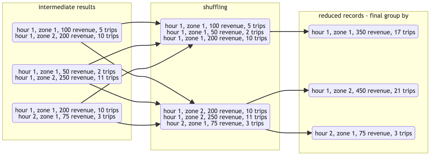
df_partitioned.write.parquet('[path_to_output_directory]', mode="overwrite")GROUP BY
Shuffling: Spark redistributes data across the cluster so that all records with the same key are grouped together. This step involves transferring data between executors or nodes, which can be resource-intensive.
Aggregation Steps:
Map Phase: Data is prepared for aggregation, organizing it into key-value pairs based on the
groupBykey.Shuffle Phase: Data is shuffled across the cluster to group records by key.
Reduce Phase: Aggregated computations (like sum, count) are performed on the grouped data.
Optimization:
Spark may perform partial aggregations before shuffling to reduce data transfer.
The final aggregation produces the result after shuffling.
Key Points:
Performance: The
groupByoperation can be costly, mainly due to the shuffle. Optimizing query performance involves minimizing the data shuffled.Data Skew: Uneven distribution of data across keys can affect performance, requiring strategies to handle skew.
Stage 1: Group results inside the partitions → temporary partition

Stage 2: Shuffle data
Reducebykey
reduceByKey in Apache Spark can help prevent memory outages by optimizing the aggregation process.
Local Reduction: Before shuffling data across the network, reduceByKey combines values with the same key within each partition. This significantly reduces the amount of data that needs to be shuffled.
Less Data Shuffled: By aggregating data locally first, reduceByKey minimizes the volume of data transferred over the network, leading to lower memory usage during the shuffle phase.
Efficiency: It directly reduces the memory footprint by ensuring that only aggregated results per key are shuffled, rather than all key-value pairs, which is what happens with groupBy() before reduction.
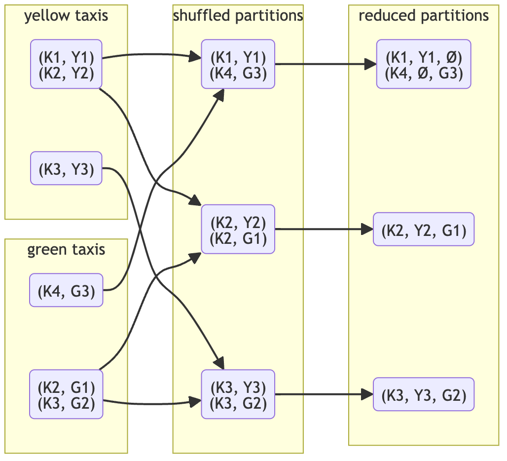
JOIN
Types of Joins
Inner Join: Returns rows with matching keys in both DataFrames.
Outer Join: Includes rows with non-matching keys.
Left Outer Join: All rows from the left DataFrame, plus matched rows from the right DataFrame.
Right Outer Join: All rows from the right DataFrame, plus matched rows from the left DataFrame.
Full Outer Join: Rows when there is a match in either DataFrame.
Cross Join: The Cartesian product of rows from both DataFrames.
Semi Join: Rows from the first DataFrame with matching keys in the second DataFrame, excluding the second DataFrame's columns.
Anti Join: Rows from the first DataFrame without matching keys in the second DataFrame.
Basic Join Syntax in PySpark
df1.join(df2, on=[key], how='join_type')Performance Tips
Shuffle Joins: Can be costly due to data shuffling across the cluster. Use them for large datasets that are distributed across nodes.

Broadcast Joins: Preferable when joining a large DataFrame with a smaller one. Broadcasting the smaller DataFrame can reduce shuffling and improve performance.


Spark in the Cloud
Pre-requisites:
Ensure you are logged into Google Cloud Platform (GCP).
If you are not logged in, follow these instructions to log in to GCP and set up your environment.
Upload data to GCS
Use gsutil to upload local data (<local_folder>) to GCS bucket.
gsutil -m cp -r <local_folder> gs://<bucket_name/destination_folder>-m: Enables multithreaded uploads for faster transfer.cp: Copies files.-r: Recursively uploads folder contents; not needed for single files.
Read data from GCS
In your terminal set up a GCS connector
download corresponding version (e.g. version 2.5.5 for Hadoop 3) of the connecter here
copy the content to your local machine (
.libdirectory for convenience)gsutil cp gs://hadoop-lib/gcs/gcs-connector-hadoop3-2.2.5.jar gcs-connector-hadoop3-2.2.5.jar
In jupyter notebook import required libraries and create a configuration object
import pyspark
from pyspark.sql import SparkSession
from pyspark.conf import SparkConf
from pyspark.context import SparkContext

credentials_location = '~/.google/credentials/google_credentials.json'

conf = SparkConf() \
    .setMaster('local[*]') \
    .setAppName('test') \
    .set("spark.jars", "./.lib/gcs-connector-hadoop3-2.2.5.jar") \
    .set("spark.hadoop.google.cloud.auth.service.account.enable", "true") \
    .set("spark.hadoop.google.cloud.auth.service.account.json.keyfile", credentials_location)
Check the path to GCP credentials and gcs connector (you can use full path)
Using the configuration settings, create and configure the context
sc = SparkContext(conf=conf)

hadoop_conf = sc._jsc.hadoopConfiguration()

hadoop_conf.set("fs.AbstractFileSystem.gs.impl",  "com.google.cloud.hadoop.fs.gcs.GoogleHadoopFS")
hadoop_conf.set("fs.gs.impl", "com.google.cloud.hadoop.fs.gcs.GoogleHadoopFileSystem")
hadoop_conf.set("fs.gs.auth.service.account.json.keyfile", credentials_location)
hadoop_conf.set("fs.gs.auth.service.account.enable", "true")
Instantiate the session
spark = SparkSession.builder \
    .config(conf=sc.getConf()) \
    .getOrCreate()
Read the remote data
df_green = spark.read.parquet('gs://bucjet_path/file_name')
Creating a Persistent Spark Cluster
When a Spark cluster is initiated within a Jupyter notebook, it ceases to exist once the notebook's kernel is halted. To maintain cluster operation beyond the notebook session, it's necessary to establish a Spark cluster using Standalone Mode.
Create a python script and follow the instructions.
CLI: In the spark install directory start the master node of a Spark cluster in Standalone Mode
./sbin/start-master.shNow you can open Spark UI on
localhost:8080with 0 workers.
Python script: Start a Spark Session with URL from Spark UI
spark = SparkSession.builder \
    .master("master-spark-URL") \
    .appName('test') \
    .getOrCreate()
master-spark-URL:
spark://.....:7077
CLI: In the spark install directory run a worker
./sbin/start-worker.sh <master-spark-URL>may be
start-slave.shin older versions of spark
CLI: Manually shut down Spark in standalone mode
-- Stop worker
./sbin/stop-worker.sh

-- Stop master node
./sbin/stop-master.sh
may be
stop-slave.shin older versions of Spark
Parametrize the script
Parse parameters from CLI
You can use argparse library to input parameters from the CLI
e.g. paths of the different input and output destinations
import argparse

parser = argparse.ArgumentParser()

parser.add_argument('--input_green', required=True)
parser.add_argument('--input_yellow', required=True)
parser.add_argument('--output', required=True)

args = parser.parse_args()

input_green = args.input_green
input_yellow = args.input_yellow
output = args.output
Parametrize different clusters with Spark submit
Different clusters have different master-spark-URLs
CLI
spark-submit \
    --master="spark://<URL>" \
    my_script.py \
        --input_green=data/pq/green/2020/*/ \
        --input_yellow=data/pq/yellow/2020/*/ \
        --output=data/report-2020
Python script
spark = SparkSession.builder \
    .appName('test') \
    .getOrCreate()

# no need to specify master URL
Dataproc Cluster
Google Cloud Dataproc is a managed service on Google Cloud Platform (GCP) designed to simplify and accelerate the deployment of Apache Spark and Hadoop clusters, enabling scalable and efficient processing of big data workloads.
Create Dataproc Cluster
Go to your GCP and navigate to Dataproc (via search bar)
Enable Cloud Dataproc API, if not enabled
Create cluster on Compute Engine
cluster name: any
location: same as your bucket’s location
cluster type: Standard
for the tutorial purpose - Single Node
Optional components
For our tutorial: Jupyter notebook, Docker
You may notice an extra VM instance under VMs; that's the Spark instance.
There are different ways to submit a job in Dataproc cluster
After submitting a job, 2 more dataproc buckets will be created: temporary and staging
Spark - GCS
Run the job with web UI
Since the connection is already pre-configured in Dataproc, we do not need to specify it as we did previously
Navigate inside you cluster and press
Submit jobJob type: PySpark
Main python file:
gs://<bucket_name>/code.pyPreliminarily upload your code to your bucket using
gsutil cpcommand
Arguments: Add required arguments as you would in the CLI
Press submit
Check the job status from the Job details page
Run the job with CLI (gcloud SDK)
Grant permission (Dataproc Hub Agent) to your service account via IAM & Admin → IAM
In your CLI run:
gcloud dataproc jobs submit pyspark \
    --cluster=<your-cluster-name> \
    --region=<region-same-as-your-bucket> \
    gs://<url-of-your-script> \
    -- \
        --param1=<your-param-value> \
        --param2=<your-param-value>
Better to submit in one code line
Spark - BigQuery
Link with code specifics template to upload export to BigQuery
set the path to bucket with dataproc temp data
spark.conf.set('temporaryGcsBucket', "dataproc-temp-...")the export from your python file (
dataframe.writeclause) should navigate to BigQuery dataset.table path# Save the data to BigQuery <dataframe_name>.write.format('bigquery') \ .option('table', '<dataset_name>.<table_name>') \ .save()If table is not present in the dataset, pyspark will create it for you
Upload your python script to GCS
Run the job with CLI
gcloud dataproc jobs submit pyspark \
  --cluster=<CLUSTER_NAME> \
  --region=<CLUSTER_REGION> \
  --jars=gs://spark-lib/bigquery/spark-bigquery-latest.jar \
  <PYSPARK_FILE_PATH_IN_GCS> \
  -- \
    --input_green=<INPUT_GREEN_PATH_IN_GCS> \
    --input_yellow=<INPUT_YELLOW_PATH_IN_GCS> \
    --output=<OUTPUT_PATH_IN_GCS>
Other notes
Streamlining Dataset Management
For more efficient data manipulation, especially with large CSV files, you can focus on a subset by selecting a specific row range:
!head -n [number_of_rows + 1] [path_to_original_csv] > [path_to_smaller_csv]To confirm the subset's size matches your requirements, check the file line count:
!wc -l [path_to_smaller_csv]Set Execution Permission for .sh File:
chmod +x <file_name.sh>View Content of Zipped (.gz) File:
zcat <file_path/file.gz> | head -n 10